OpenCV image processing using Python

What we need to get started with OpenCv...

We need to import few libraries given below and are available in Google Colab, independent installations may be required for other platforms.

1. Imports required

from scipy.spatial import distance as dist
from imutils import perspective
from imutils import contours
import numpy as np
import argparse
import imutils
import cv2
import matplotlib.pyplot as plt
from google.colab.patches import cv2_imshow

2. Next we import an image and get its details

mg = cv2.imread(r'/content/parrot.jpg',cv2.IMREAD_UNCHANGED)
height = img.shape[0]  
width = img.shape[1]  
channels = img.shape[2]  
size1 = img.size
cv2_imshow(img)
print('Image Height       : ',height)  
print('Image Width        : ',width)  
print('Number of Channels : ',channels)  
print('Image Size  :', size1)

Remember we are using Colab and it uses its own snippets.

3. First lets try to get distance between two pixels

pixel = img[100,100]
pixel1 = img[200,200]
pixel_diff= pixel1-pixel  
print("The difference between the two pixels is :",pixel_diff)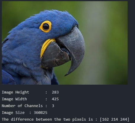

4. Next lets try Point processing in the spatial domain on Image, Image Negatives and Power-Law (Gamma) Transformation.

Negative

print("Part A : Negative of the image")
plt.imshow(img)
plt.show()
# negative transformed image
color = ('b', 'g', 'r')    
plt.show()

Power-Law (Gamma) Transformation

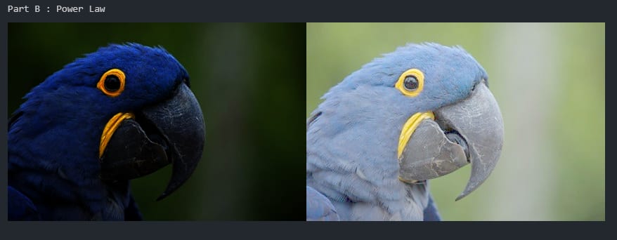
print("Part B : Power Law ")
img = cv2.imread('/content/parrot.jpg', cv2.IMREAD_UNCHANGED)
gamma_two_point_two = np.array(255*(img/255)**2.2,dtype='uint8')

# Similarly, Apply Gamma=0.4 
gamma_point_four = np.array(255*(img/255)**0.4,dtype='uint8')

# Display the images in subplots
img3 = cv2.hconcat([gamma_two_point_two,gamma_point_four])
cv2_imshow(img3)

We used hconcat for displaying results together.

5. lets try some Point processing in the spatial domain.

Contrast stretching

print("Part C : Gray-level slicing, Contrast stretching")
img = cv2.imread('/content/parrot.jpg', cv2.IMREAD_UNCHANGED)
def pixelVal(pix, r1, s1, r2, s2):
    if (0 <= pix and pix <= r1):
        return (s1 / r1)*pix
    elif (r1 < pix and pix <= r2):
        return ((s2 - s1)/(r2 - r1)) * (pix - r1) + s1
    else:
        return ((255 - s2)/(255 - r2)) * (pix - r2) + s2
r1 = 70
s1 = 0
r2 = 140
s2 = 255
pixelVal_vec = np.vectorize(pixelVal)

# Apply contrast stretching.
contrast_stretched = pixelVal_vec(img, r1, s1, r2, s2)

print("Constrat Strethcing :")
# Save edited image.
cv2_imshow(contrast_stretched)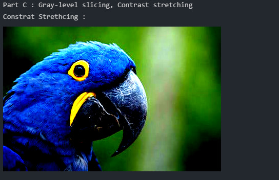

Gray-Level Slicing

class pointProcessing:
 def slicedGreyScale(self,image):
 # T1 and T2 Represent Lower and Upper Threshold Value
  T1 = 100
  T2 = 200
  h, w, c = img.shape
  img_thresh_back = np.zeros((h,w), dtype=np.uint8)
  for i in range(h):
    for j in range(w):
      if (T1 < image[i,j] and image[i,j] < T2):
        img_thresh_back[i,j]= 255
      else:
        img_thresh_back[i,j]= image[i,j]
  cv2_imshow(img_thresh_back)
pointObj= pointProcessing()
pointObj.slicedGreyScale(img)

6. Nearest neighbour Interpolation & Bilinear Interpolation.

Use of Average neighbour value and Bilinear

#Nearest neighbor Interpolation Using cv2.resize()Python
near_img = cv2.resize(img,None, fx = 2, fy = 2, interpolation = cv2.INTER_NEAREST)
cv2_imshow(near_img)

# Bilinear Interpolation 
bilinear_img = cv2.resize(img,None, fx = .5, fy = .5, interpolation = cv2.INTER_LINEAR)
cv2_imshow(bilinear_img)

7. Lets try other operations available in OpenCV

• Arithmetic operations — Addition, Division
• Logical Operations on Binary Image — XOR, NOT
• Geometrical Operations — Rotation, Affine Translation
• Statistical operations — Mean, Variance

Addition and Division -

print("A : Addition and Division :")
img1 = cv2.imread('/content/parrot.jpg')
img2 = cv2.imread('/content/bg.jpg')
dst = cv2.addWeighted(img1,0.3,img2,0.7,0)
#Div
div = cv2.divide(img1, img2)
AddDiv = cv2.hconcat([dst,div])
cv2_imshow(AddDiv)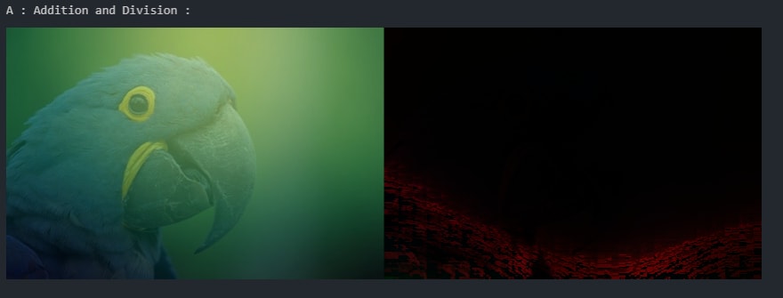

XOR and NOT

print("B : Xor and Not Operations :")
#XOR function
bitwiseXor = cv2.bitwise_xor(img1, img2)
#NOT function
bitwiseNot = cv2.bitwise_not(img1)
#concat
img5 = cv2.hconcat([bitwiseXor,bitwiseNot])
cv2_imshow(img5)

Rotation and Affine Translation

print("C : Geometric Operations :")
print("Rotation and Affine Translation :")
#Rotation
image = cv2.rotate(img1, cv2.cv2.ROTATE_90_CLOCKWISE)
cv2_imshow(image)
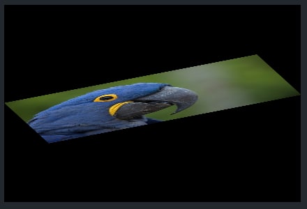
#Affine Translation
srcTri = np.array( [[0, 0], [img1.shape[1] - 1, 0], [0, img1.shape[0] - 1]] ).astype(np.float32)
dstTri = np.array( [[0, img1.shape[1]*0.33], [img1.shape[1]*0.85, img1.shape[0]*0.25], [img1.shape[1]*0.15, img1.shape[0]*0.7]] ).astype(np.float32)
warp_mat = cv2.getAffineTransform(srcTri, dstTri)
warp_dst = cv2.warpAffine(img1, warp_mat, (img1.shape[1], img1.shape[0]))
# Rotating the image after Warp
center = (warp_dst.shape[1]//2, warp_dst.shape[0]//2)
angle = -50
scale = 0.6
rot_mat = cv2.getRotationMatrix2D( center, angle, scale )
warp_rotate_dst = cv2.warpAffine(warp_dst, rot_mat, (warp_dst.shape[1], warp_dst.shape[0]))
cv2_imshow(warp_dst)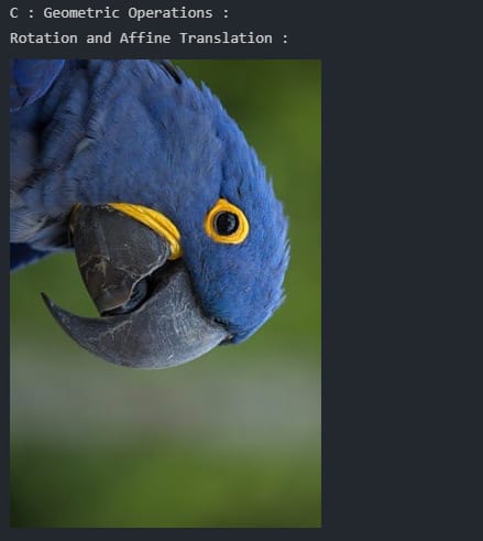

Mean and Variance

print("D : Mean, Variance :")
#Mean of img1 and img2 
img7 = (img1+img2) * 0.5;
cv2_imshow(img7)
#Variance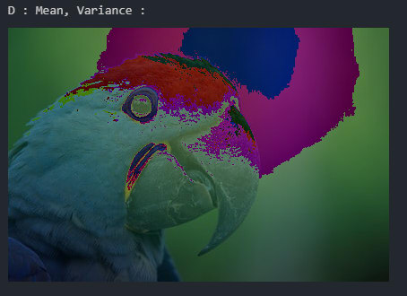

Image interpolation : Down Sampling

print("E : Image interpolation : Down Sampling")
ds = cv2.pyrDown(img1)
cv2_imshow(ds)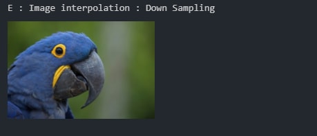

As of now, We have covered the basics of OpenCV