Logistic Regression at a glance

What is Logistic Regression?

In problems where a discrete value (0, 1, 2...) is to be predicted based on some input values, Logistic Regression can be very handy. Examples of such problems are - detecting if a student will be selected in a graduate program depending on his profile, or if an Instagram account has been hacked depending on its recent activity. These problems can be solved by "Supervised Classification Models", one of which is Logistic Regression.

To build such a model, we need to supply the model with some training data, ie, samples of various data values as inputs and their corresponding discrete valued outputs. The input can be defined in terms of several independent features on which the output depends. For instance, if we take the problem of predicting if an Instagram account has been hacked, we can define some independent features such as "activity time", "5 recent texts", "5 recent comments", "10 recently liked posts" and so on. Using this input training data, the model essentially "learns" what the traits of a hacked Instagram account and uses this knowledge to make predictions on other accounts to check if they are hacked.

However, you and I both know it is not that simple. So what goes on behind this black box?

Diving into the math!

First, let us set some notations.

If we have "n" features and "m" training samples, they can be arranged in an "n*m" matrix consisting of training samples as column vectors horizontally stacked together as given in the image below. Let us call this matrix X.

It has a corresponding vector which contains the discrete valued outputs for each training sample. It is a single column vector of dimension m*1. Let us call this vector Y.

With the notations set and out of the way, let's get to the heart of logistic regression!

The equations

We first calculate the probability that the output value of a particular input is 1 (given that the set of output labels = {0, 1}), which is also denoted as given below -

First, a hypothesis value Z is calculated by finding the transpose of a weight parameter W (column vector of dimensions n*1) multiplied with the matrix X (matrix of dimensions n*m), and then added to another bias parameter b (row vector of dimension 1*m). This gives us Z, a row vector of dimension 1*m.

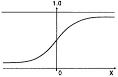
Then, an irregularity function "sigmoid" is applied to Z to give us the predicted probability for that particular input set. It outputs a value between 0 and 1 as shown in the figure below.
The equation for the sigmoid function is -

Thus, our final equation becomes -
This gives us a row vector of dimension 1*m. It has the predicted probabilities of the m-training samples. When the probability is greater than 0.5, it is classified as output 1, and if the probability is less than 0,5, then it is classified as output 0.

Here, the parameters W and b are trained and set to optimal values that give the highest accuracy in predicting the probability that the output is 1. A loss value is calculated for each training example, and depending on the value, the parameters are adjusted to give better results and reduce this loss value. This is essentially what is referred to as "training" a model. A low loss value suggests that the model has been successfully trained (or that the model is overfitting, but that is a concept for another blog 😁). This loss value is calculated by the equation -

Thus, we see that -

Using the loss function, we calculate the cost function, which is an addition of all the loss function values over all the training examples. It is calculated using the formula below -

Now, to adjust the values of the parameters W and b, we use the famous gradient descent algorithm (which is also for another blog 😁). This formula is given below -

This formula comes from the gradient descent algorithm. Here, the parameter alpha is called learning rate. A large learning rate causes large adjustments in parameters while a small learning rate causes smaller adjustments. It can be tuned according to our requirements.

And viola! That wraps up one iteration of training our Logistic Regression Model! Connect enough of these together with slight modification, and we get a neural net!

Hope you enjoyed reading this, thank you for reading till the end!