26
Build a Spam Classifier in python
Ever since the introduction of emails, humankind has been plagued by spam messages. Any promotional messages or advertisements that end up in our inbox can be categorised as spam as they don't provide any value and often irritates us.
We will make use of the SMS spam classification data.
The SMS Spam Collection is a set of SMS tagged messages that have been collected for SMS Spam research. It contains one set of SMS messages in English of 5,574 messages, tagged according to being ham (legitimate) or spam.
The data was obtained from UCI’s Machine Learning Repository, alternatively, I have also uploaded the dataset and completed Jupiter notebook onto my GitHub repo.
Data processing
Building a classification model
%matplotlib inline
import matplotlib.pyplot as plt
import csv
import sklearn
import pickle
from wordcloud import WordCloud
import pandas as pd
import numpy as np
import nltk
from nltk.corpus import stopwords
from sklearn.feature_extraction.text import CountVectorizer, TfidfTransformer
from sklearn.tree import DecisionTreeClassifier
from sklearn.model_selection import GridSearchCV,train_test_split,StratifiedKFold,cross_val_score,learning_curve
please note! You might find that I have reimported some of these packages again later in the article, it is just for ease of use if I ever have to use those code blocks again in future projects, you may omit those.😉
data = pd.read_csv('dataset/spam.csv', encoding='latin-1')
data.head()
From the above figure, we can see that there are some unnamed columns and the label and text column name is not intuitive so let's fix those in this step.
data = data.drop(["Unnamed: 2", "Unnamed: 3", "Unnamed: 4"], axis=1)
data = data.rename(columns={"v2" : "text", "v1":"label"})
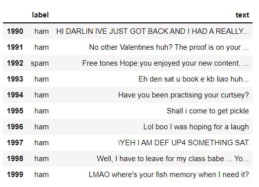
data[1990:2000]
now that the data is looking pretty, let's move on.
data['label'].value_counts()

//OUTPUT
ham     4825
spam     747
Name: label, dtype: int64If you are completely new to NLTK and Natural Language Processing(NLP) I would recommend checking out this short article before continuing.
Introduction to Word Frequencies in NLP
Introduction to Word Frequencies in NLP
# Import nltk packages and Punkt Tokenizer Models
import nltk
nltk.download("punkt")
import warnings
warnings.filterwarnings('ignore')ham words are the opposite of spam in this dataset, 🤷♂️ yeah I also don't have any clue why it is so.
ham_words = ''
spam_words = ''
# Creating a corpus of spam messages
for val in data[data['label'] == 'spam'].text:
text = val.lower()
tokens = nltk.word_tokenize(text)
for words in tokens:
spam_words = spam_words + words + ' '
# Creating a corpus of ham messages
for val in data[data['label'] == 'ham'].text:
text = text.lower()
tokens = nltk.word_tokenize(text)
for words in tokens:
ham_words = ham_words + words + ' 'let's use the above functions to create Spam word cloud and ham word cloud.
spam_wordcloud = WordCloud(width=500, height=300).generate(spam_words)
ham_wordcloud = WordCloud(width=500, height=300).generate(ham_words)
#Spam Word cloud
plt.figure( figsize=(10,8), facecolor='w')
plt.imshow(spam_wordcloud)
plt.axis("off")
plt.tight_layout(pad=0)
plt.show()
#Creating Ham wordcloud
plt.figure( figsize=(10,8), facecolor='g')
plt.imshow(ham_wordcloud)
plt.axis("off")
plt.tight_layout(pad=0)
plt.show()
from the spam word cloud, we can see that "free" is most often used in spam.
Now, we can convert the
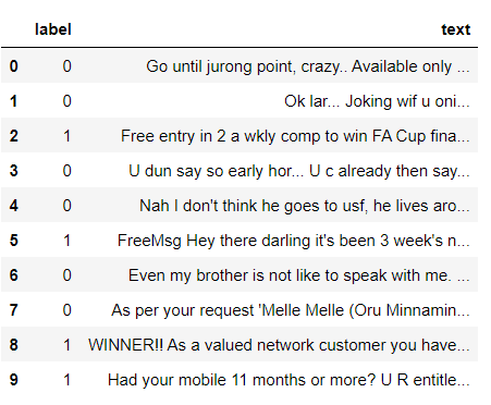
spam and ham into 0 and 1 respectively so that the machine can understand.data = data.replace(['ham','spam'],[0, 1])
data.head(10)
Punctuation and stop words do not contribute anything to our model, so we have to remove them. Using NLTK library we can easily do it.
import nltk
nltk.download('stopwords')

#remove the punctuations and stopwords
import string
def text_process(text):

    text = text.translate(str.maketrans('', '', string.punctuation))
    text = [word for word in text.split() if word.lower() not in stopwords.words('english')]

    return " ".join(text)

data['text'] = data['text'].apply(text_process)
data.head()
Now, create a data frame from the processed data before moving to the next step.
text = pd.DataFrame(data['text'])
label = pd.DataFrame(data['label'])we can convert words to vectors using either Count Vectorizer or by using TF-IDF Vectorizer.
TF-IDF is better than Count Vectorizers because it not only focuses on the frequency of words present in the corpus but also provides the importance of the words. We can then remove the words that are less important for analysis, hence making the model building less complex by reducing the input dimensions.
I have included both methods for your reference.
## Counting how many times a word appears in the dataset

from collections import Counter

total_counts = Counter()
for i in range(len(text)):
    for word in text.values[i][0].split(" "):
        total_counts[word] += 1

print("Total words in data set: ", len(total_counts))

// OUTPUT
Total words in data set:  11305
# Sorting in decreasing order (Word with highest frequency appears first)
vocab = sorted(total_counts, key=total_counts.get, reverse=True)
print(vocab[:60])
// OUTPUT
['u', '2', 'call', 'U', 'get', 'Im', 'ur', '4', 'ltgt', 'know', 'go', 'like', 'dont', 'come', 'got', 'time', 'day', 'want', 'Ill', 'lor', 'Call', 'home', 'send', 'going', 'one', 'need', 'Ok', 'good', 'love', 'back', 'n', 'still', 'text', 'im', 'later', 'see', 'da', 'ok', 'think', 'Ì', 'free', 'FREE', 'r', 'today', 'Sorry', 'week', 'phone', 'mobile', 'cant', 'tell', 'take', 'much', 'night', 'way', 'Hey', 'reply', 'work', 'make', 'give', 'new']# Mapping from words to index
vocab_size = len(vocab)
word2idx = {}
#print vocab_size
for i, word in enumerate(vocab):
word2idx[word] = I# Text to Vector
def text_to_vector(text):
word_vector = np.zeros(vocab_size)
for word in text.split(" "):
if word2idx.get(word) is None:
continue
else:
word_vector[word2idx.get(word)] += 1
return np.array(word_vector)# Convert all titles to vectors
word_vectors = np.zeros((len(text), len(vocab)), dtype=np.int_)
for i, (_, text_) in enumerate(text.iterrows()):
word_vectors[i] = text_to_vector(text_[0])
word_vectors.shape
// OUTPUT
(5572, 11305)#convert the text data into vectors
from sklearn.feature_extraction.text import TfidfVectorizer
vectorizer = TfidfVectorizer()
vectors = vectorizer.fit_transform(data['text'])
vectors.shape
// OUTPUT
(5572, 9376)#features = word_vectors
features = vectors#split the dataset into train and test set
X_train, X_test, y_train, y_test = train_test_split(features, data['label'], test_size=0.15, random_state=111)#import sklearn packages for building classifiers
from sklearn.linear_model import LogisticRegression
from sklearn.svm import SVC
from sklearn.naive_bayes import MultinomialNB
from sklearn.tree import DecisionTreeClassifier
from sklearn.neighbors import KNeighborsClassifier
from sklearn.ensemble import RandomForestClassifier
from sklearn.metrics import accuracy_score#initialize multiple classification models
svc = SVC(kernel='sigmoid', gamma=1.0)
knc = KNeighborsClassifier(n_neighbors=49)
mnb = MultinomialNB(alpha=0.2)
dtc = DecisionTreeClassifier(min_samples_split=7, random_state=111)
lrc = LogisticRegression(solver='liblinear', penalty='l1')
rfc = RandomForestClassifier(n_estimators=31, random_state=111)#create a dictionary of variables and models
clfs = {'SVC' : svc,'KN' : knc, 'NB': mnb, 'DT': dtc, 'LR': lrc, 'RF': rfc}#fit the data onto the models
def train(clf, features, targets):
clf.fit(features, targets)
def predict(clf, features):
return (clf.predict(features))pred_scores_word_vectors = []
for k,v in clfs.items():
train(v, X_train, y_train)
pred = predict(v, X_test)
pred_scores_word_vectors.append((k, [accuracy_score(y_test , pred)]))pred_scores_word_vectors
// OUTPUT
[('SVC', [0.9784688995215312]),
('KN', [0.9330143540669856]),
('NB', [0.9880382775119617]),
('DT', [0.9605263157894737]),
('LR', [0.9533492822966507]),
('RF', [0.9796650717703349])]#write functions to detect if the message is spam or not
def find(x):
if x == 1:
print ("Message is SPAM")
else:
print ("Message is NOT Spam")newtext = ["Free entry"]
integers = vectorizer.transform(newtext)x = mnb.predict(integers)
find(x)
// OUTPUT
Message is SPAMfrom sklearn.metrics import confusion_matrix
import seaborn as sns
# Naive Bayes
y_pred_nb = mnb.predict(X_test)
y_true_nb = y_test
cm = confusion_matrix(y_true_nb, y_pred_nb)
f, ax = plt.subplots(figsize =(5,5))
sns.heatmap(cm,annot = True,linewidths=0.5,linecolor="red",fmt = ".0f",ax=ax)
plt.xlabel("y_pred_nb")
plt.ylabel("y_true_nb")
plt.show()
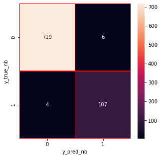
from the confusion matrix, we can see that the Naive Bayes model is balanced. That's it !!
we have successfully created a spam classifier. 🎉🎉
we have successfully created a spam classifier. 🎉🎉
You can find the code and dataset here.
If you liked this tutorial please do share it with your friends or on social media!
🎃 In case of any suggestions, corrections or if you want to have a chat about data science? Ping me on Twitter
26
