21
Detecting emotions from speech with neural networks in Python
During a data science bootcamp, I built a machine learning model that detects emotions from speech (pre-recorded files and live-recorded voices). The code is available on my GitHub.
This has been one of the most challenging projects I've worked on, but also the most exciting. In this post, I'll walk you through my project: from planning adn choosing a data set to building machine learning models and evaluating their performance.
First and foremost, I designed a project plan, after having a brief look at the data set. From my work experience and the assignments completed in the past three months, I've learned that this step is crucial for the success of a coding project. Planning helps me (and the team) organize my ideas, break down the big project into smaller tasks, identify issues, and track the progress -- and not despair at the amount of work to be done in a short time.
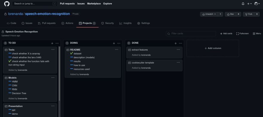
For this purpose, I created a simple Kanban board directly in the GitHub repository of my project, so that I have the code and tasks in one place.

To create a project board linked to a repository in GitHub:
- In your desired repository, click on the tab
Projects, then onCreate project. - Enter the
Project board name. - (Optional) Enter a
Descriptionof the project and select aProject template. - Click on
Create project.
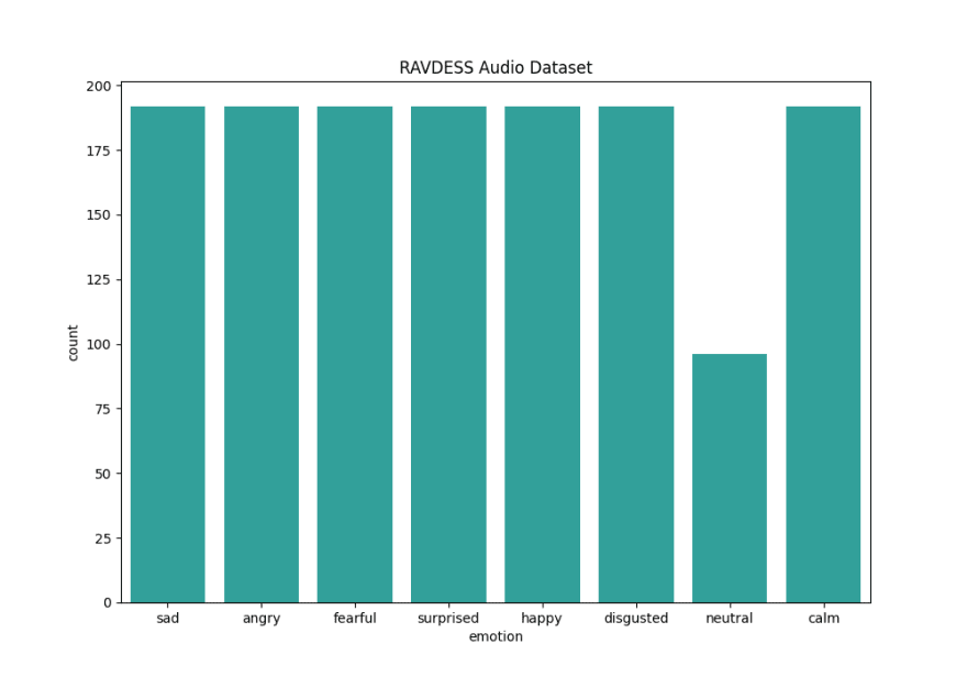
I used the RAVDESS data set, which contains 1440 audio files. These are voice recordings of 24 actors (12 male, 12 female) who say two sentences in two different intensities (normal and strong) with eight intonations that express different emotions: calm, happy, sad, angry, fearful, surprised, disgusted, and neutral. There are 192 recordings for each emotion, except for neutral, which doesn't have recordings in strong intensity.
To sum up, the original RAVDESS data set includes:
- 1440 recordings
- 24 speakers
- 12 male, 12 female
- 2 sentences
- 2 intensities
- 8 intonations / emotions
- 192 recordings for 7 emotions
- 96 recordings for 1 emotion

The data set was imbalanced, so I used the RandomOversample method to create new features for the neutral class.
def oversample(X, y):
    X = joblib.load("speech_emotion_recognition/features/X.joblib")
    y = joblib.load("speech_emotion_recognition/features/y.joblib")
    print(Counter(y))

    oversample = RandomOverSampler(sampling_strategy="minority")
    X_over, y_over = oversample.fit_resample(X, y)

    X_over_save, y_over_save = "X_over.joblib", "y_over.joblib"
    joblib.dump(X_over, os.path.join("speech_emotion_recognition/features/", X_over_save))
    joblib.dump(y_over, os.path.join("speech_emotion_recognition/features/", y_over_save))
Oversampling added 96 new datapoints, so in the end I had 1536 audio files to work with.
Another imbalance was gender-related: there were slightly more recordings by males and in normal intensity. I didn't deal with this imbalance because it wasn't significant to my project, since I only wanted to predict the emotion. However, it would be interesting to explore in the future.
There are many features that can be extracted from audio files, but I decided to work with the Mel Frequency Cepstral Coefficient (MFCC).
Mel-frequency cepstrum (MFC) is a representation of the short-term power spectrum of a sound, based on a linear cosine transform of a log power spectrum on a nonlinear mel scale of frequency. Mel-frequency cepstral coefficients (MFCCs) are coefficients that collectively make up an MFC.
The difference between the cepstrum and the mel-frequency cepstrum is that in the MFC, the frequency bands are equally spaced on the mel scale, which approximates the human auditory system's response more closely than the linearly-spaced frequency bands used in the normal spectrum. This frequency warping can allow for better representation of sound, for example, in audio compression.
To extract the MFCC from the audio files, I used the Python library librosa:
def extract_features(path, save_dir):
    feature_list = []

    start_time = time.time()
    for dir, _, files in os.walk(path):
        for file in files:
            y_lib, sample_rate = librosa.load(
                os.path.join(dir, file), res_type="kaiser_fast"
            )
            mfccs = np.mean(
                librosa.feature.mfcc(y=y_lib, sr=sample_rate, n_mfcc=40).T, axis=0
            )

            file = int(file[7:8]) - 1
            arr = mfccs, file
            feature_list.append(arr)

    print("Data loaded in %s seconds." % (time.time() - start_time))

    X, y = zip(*feature_list)
    X, y = np.asarray(X), np.asarray(y)
    print(X.shape, y.shape)

    X_save, y_save = "X.joblib", "y.joblib"
    joblib.dump(X, os.path.join(save_dir, X_save))
    joblib.dump(y, os.path.join(save_dir, y_save))

    return "Preprocessing completed."
The visual representation of MFCC looks like this:

I trained three different neural networks models on the MFCC and emotion labels:
-
Multi-Layer Perceptron (MLP)
def mlp_classifier(X, y): X_train, X_test, y_train, y_test = train_test_split( X, y, test_size=0.2, random_state=42 ) mlp_model = MLPClassifier( hidden_layer_sizes=(100,), solver="adam", alpha=0.001, shuffle=True, verbose=True, momentum=0.8, ) -
Convolutional Neural Network (CNN)
def cnn_model(X, y): X_train, X_test, y_train, y_test = train_test_split( X, y, test_size=0.2, random_state=42 ) x_traincnn = np.expand_dims(X_train, axis=2) x_testcnn = np.expand_dims(X_test, axis=2) model = Sequential() model.add(Conv1D(16, 5, padding="same", input_shape=(40, 1))) model.add(Activation("relu")) model.add(Conv1D(8, 5, padding="same")) model.add(Activation("relu")) model.add( Conv1D( 8, 5, padding="same", ) ) model.add(Activation("relu")) model.add(BatchNormalization()) model.add(Activation("relu")) model.add(Flatten()) model.add(Dense(8)) model.add(Activation("softmax")) model.compile( loss="categorical_crossentropy", optimizer="adam", metrics=["accuracy"], ) cnn_history = model.fit( x_traincnn, y_train, batch_size=50, epochs=100, validation_data=(x_testcnn, y_test), ) -
Long Short-Term Memory (LSTM)
def lstm_model(X, y):
X_train, X_test, y_train, y_test = train_test_split(
    X, y, test_size=0.2, random_state=42
)
X_train_lstm = np.expand_dims(X_train, axis=2)
X_test_lstm = np.expand_dims(X_test, axis=2)

lstm_model = Sequential()
lstm_model.add(LSTM(64, input_shape=(40, 1), return_sequences=True))
lstm_model.add(LSTM(32))
lstm_model.add(Dense(32, activation="relu"))
lstm_model.add(Dropout(0.1))
lstm_model.add(Dense(8, activation="softmax"))

lstm_model.compile(
    optimizer="adam", loss="categorical_crossentropy", metrics=["accuracy"]
)

lstm_model.summary()
lstm_history = lstm_model.fit(X_train_lstm, y_train, batch_size=32, epochs=100)
After several iterations of tweaking the hyperparameters, I found that generally the models performed better with low learning rates (0.001), adam optimizer, and less layers. All models overfit (they couldn't generalize on unseen data), but this seems to be a common issue in neural networks and on audio data.
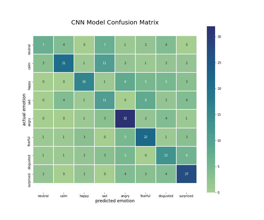
As expected, MLP had the lowest accuracy, since it's a very basic model (a simple feed-forward artificial neural network). CNN and LSTM had similar train accuracy (80%), but CNN performed better on test data (60%) than LSTM (51%). To give you some context, state-of-the-art models for speech classification have an accuracy of 70-80%, so I was quite happy with my CNN model accuracy.

It was particularly interesting to look at the actual vs. predicted emotions, to see what emotions were misclassified. From the correlations matrices of CNN and LSTM, I noticed that both models misclassified emotions that sound similar or are ambiguous (even for humans), like sad-calm or angry-happy.


The exciting part was to make predictions on new data, more specifically on movie sound clips and my own voice in real-time. To record my voice, I used the Python library sounddevice:
import soundfile as sf
import sounddevice as sd
from scipy.io.wavfile import write


def record_voice():
    fs = 44100  # Sample rate
    seconds = 3  # Duration of recording
    # sd.default.device = "Built-in Audio"  # Speakers full name here

    print("Say something:")
    myrecording = sd.rec(int(seconds * fs), samplerate=fs, channels=2)
    sd.wait()  # Wait until recording is finished
    write("speech_emotion_recognition/recordings/myvoice.wav", fs, myrecording)
    print("Voice recording saved.")
I then tested the CNN and LSTM models on pre- and live-recorded audio files:
def make_predictions(file):
    cnn_model = keras.models.load_model(
        "speech_emotion_recognition/models/cnn_model.h5"
    )
    lstm_model = keras.models.load_model(
        "speech_emotion_recognition/models/lstm_model.h5"
    )
    prediction_data, prediction_sr = librosa.load(
        file,
        res_type="kaiser_fast",
        duration=3,
        sr=22050,
        offset=0.5,
    )

    mfccs = np.mean(
        librosa.feature.mfcc(y=prediction_data, sr=prediction_sr, n_mfcc=40).T, axis=0
    )
    x = np.expand_dims(mfccs, axis=1)
    x = np.expand_dims(x, axis=0)
    predictions = lstm_model.predict_classes(x)

    emotions_dict = {
        "0": "neutral",
        "1": "calm",
        "2": "happy",
        "3": "sad",
        "4": "angry",
        "5": "fearful",
        "6": "disgusted",
        "7": "surprised",
    }

    for key, value in emotions_dict.items():
        if int(key) == predictions:
            label = value

    print("This voice sounds", predictions, label)
Both models identified the correct or plausible emotion from recorded speech!
It was super exciting to work on this project and I'm already thinking of improving and extending it in some ways:
- Try other models (not necessarily neural networks).
- Extract other audio features to see if they are better predictors than the MFCC.
- Train on larger data sets, since 1500 files and only 200 samples per emotion is not enough.
- Train on natural data, i.e. on recordings of people speaking in unstaged situations, so that the emotional speech sounds more realistic.
- Train on more diverse data, i.e. on recordings of people of different cultures and languages. This is important because the expression of emotions varies across cultures and is influenced also by individual experiences.
- Combine speech with facial expressions and text (speech-to-text) for multimodal sentiment analysis.
21
