22
Linear Regression using Normal Equation
Linear Regression is the first algorithm in the Demystifying Machine Learning series and in this article we'll be discussing Linear Regression using Normal equation. This article covers what is Linear Regression, how it works, the maths behind the normal equation method, fixing some edge cases, handling overfitting and code implementation.
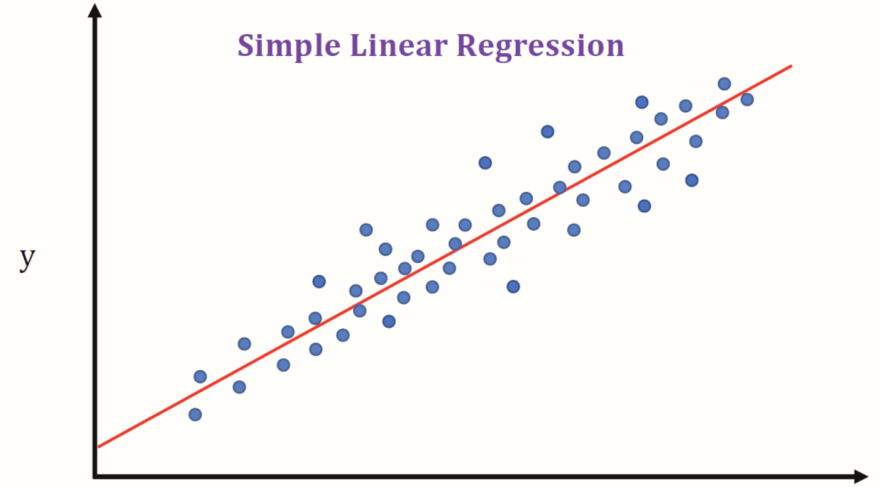
Linear Regression in simple terms is fitting the best possible linear hypothesis (a line or a hyperplane) on the data having a linear relationship so that we can predict the new unknown data point with the least possible error. It's not necessary to have a linear relationship in data but having such can lead to approximately close predictions. For a reference take a look at the below representation.

In the above picture, only 1 feature (along the x-axis) and the target (along the y-axis) is displayed just for the sake of simplicity and we can see that the red line is fitting the data very nicely covering most of the variance.
One thing is to be noted that we call it Linear Regression but it's not always fitting a line, we call it hypothesis or hyperplane. If we have N-Dimensional data (data having N number of features) then we can fit a hyperplane of atmost N-Dimensions.
Let's take a very simpler problem and dataset to derive and mimic the algorithm we are going to use in Linear Regression.
Assume we have a dataset in which we have only 1 feature say x and target as y such that x = [1,2,3] and y = [1,2,2] and we are going to fit the best possible line on this dataset.

In the above plot, we can see that the feature is displayed on the x-axis and the target is along y-axis and the blue line is the best possible hypothesis through the points. Now all we need to understand is how to come up with this best possible hypothesis that is the above blue line in our case.
The equation of any line is in the format of y = wx + b where w is the slope and b is the intercept. In machine learning lingo we call w as weight and b as bias. For above line it came out to be w = 0.5 and *b = 0.667 * (Don't worry! we'll see how).
Now ultimately we can say that somehow we need to calculate the weight and bias term/terms (since 'x' is already known to us) for hypothesis and then we could use them to get the line's equation.
We are going to use some Linear Algebra concepts for finding the right weight and bias terms for our data.
Let say the weight and bias terms are w and b respectively. So we can write each data point (x, y) as :

we can write the above equations as a system of equations using matrices as Xθ = Y where X is input / feature matrix, θ is matrix for unknowns and Y is the target matrix as:

Great, Now all we need is to solve this system of equations and get the w and b terms.
Wait there's a problem. We can't solve the above system of equations because target matrix Y does not lie in the column space of input matrix X. In simple terms, if we see the previous graph again then we can notice that our data points are not collinear i.e. they don't lie on the line so and that's why we can't find the w and b for the above system of equations.
And if we think for a moment then it sounds right because in Linear Regression we fit a hypothesis to predict the target for some input with the least possible error. We do not intend to predict the exact target.
So what we can do here? We can't solve the above system of equations because Y is not in the column space of X. So instead we can project the Y onto the column space of X. It is exactly equivalent to projecting one vector onto another.

In the above representation, a and b are two vectors and the a1 is the projection of vector a onto b. With this, we can see that now we have the component of vector a that lies in the vector space of b.
We can achieve the component of Y that lies in the column space of X by doing inner product (also known as dot product).
The inner product of two vectors a and b can be found by calculating aTb


The above equation is known as Normal equation. Now we have the formula to find our matrix θ, let's use it and calculate the w and b.

from the above last equation we have our w = 0.5 and b = 2/3 (0.6667) and we can check from the equation of blue line that our w and b are exactly correct. That's how we can get the weights and bias terms for our perfect hypothesis using the Normal equation.
Now it's time to get our hands dirty with code implementation and make our algorithm work for real datasets. In this section we're going to create a class NormalLinearRegression to handle all the computations for us and return the optimal values of weights.
Note: All the code files can be found on Github through this link.
And it's highly recommended to follow the notebook along with this section for better understanding.
class NormalLinearRegression:
    def __init__(self) -> None:
        self.X = None
        self.Y = None
        self.theta = None

    def fit(self,x,y):
        """
        Returns the optimal weights.
        parameters:
            x : input/feature matrix
            y : target matrix

        Returns:
            theta: Array of the optimal value of weights.

        """
        self.X = x

        if self.X.ndim == 1: # adding extra dimension, if X is a 1-D array
            self.X = self.X.reshape(-1,1)

        # adding extra column of 1s for the bias term
        self.X = np.concatenate([np.ones((self.X.shape[0], 1)), self.X], axis=1)

        self.Y = y
        self.theta = np.zeros((self.X.shape[1],1))

        self.theta = self.calculate_theta()
        self.theta = self.theta.reshape(-1,1)

        return self.theta

    def predict(self, x):
        """
        Returns the predicted target.
        parameters:
            x : test input/feature matrix

        Returns:
            y:  predicted target value.

        """
        x = np.array(x) # converting list to numpy array
        if x.ndim == 1:
            x = x.reshape(1,-1) # adding extra dimension in front
        x = np.concatenate([np.ones((x.shape[0],1)), x], axis=1)
        return np.dot(x,self.theta)

    def calculate_theta(self):
        """
        Calculate the optimal weights.
        parameters: None
        Returns:
            theta_temp: Array containing the calculated value of weights

        """
        y_projection = np.dot(self.X.T, self.Y)
        cov = np.dot(self.X.T, self.X)
        cov_inv = np.linalg.pinv(cov)
        theta_temp = np.dot(cov_inv, y_projection)

        return theta_temp
Code is pretty self-explanatory and I added comments wherever I found necessary but still, I want to point out a few things. We are adding an extra column of 1s to X for the bias term. Since our theta matrix had both weight and bias terms so we just added an extra column of 1s so that matrix multiplication handles the addition of bias term.
We are going to test our hypothesis on two datasets. Our first dataset contains 2 columns in which the first one (only feature) is the population of a city (in 10,000s) and the second column is the profit of a food truck in that city (in $10,000s). A negative value for profit indicates a loss. Let's visualize it on the graph.

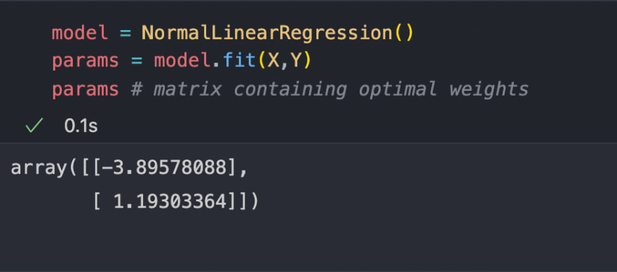
Now let's use our NormalLinearRegression class to find the best hypothesis to fit on our data.

Great now let's find the predictions using the params. Class NormalLinearRegression had a method predict that we can use to get the predictions and after that, we can use them to draw the hypothesis as shown below.

Okay, our hypothesis looks pretty nice. Now let's take a dataset that has multiple features, for the sake of graphical representation our next dataset contains a training set of housing prices in Portland, Oregon. The first column is the size of the house (in square feet), the second column is the number of bedrooms, and the third column is the price of the house. So in this dataset, we have 2 features and 1 target. Let's visualize it on the graph.

If you're wondering how I plot them, just visit the repo for this algorithm through this link and you'll find the notebook where all the implementations are already done for you.
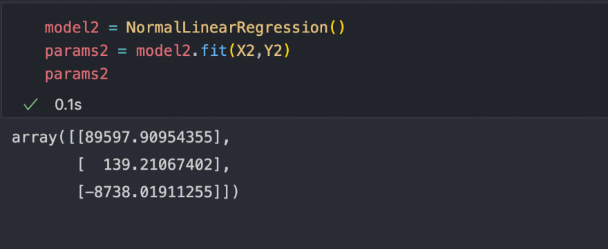
Now let's find the weights of the best hypothesis for this dataset.

Awesome, now let's find the predictions and plot the hypothesis for this dataset using the predict method of our class.

Yeah I know, it looks messy but we can uniform it as:

Now the thing to be noted is that it's not a straight line, plotting a 3D graph over a 2D surface may give a feel that it's a line but it's not. It's an N-1dimensional hyperplane and in our case, it's a 2D plane.
Great work people, so far we designed our own Linear Regression algorithm using a Normal equation and tested it on 2 datasets with single and multiple features, you can even try it on your custom dataset to see how it works. So far so good.
BUT still, there's an edge case is left, let's handle it in the next section.
When we are deriving the Normal equation, we assumed that (XTX) to be invertible and then we calculated its inverse to find the matrix θ. But what if it's not invertible?
Let's discuss the cases when it cannot be invertible:-
- (XTX) is not a square matrix
- The columns or rows of (XTX) are not independent
The 1st case is obviously wrong, let's see how?
Suppose the dimensions of X are (m,n) then the dimensions of XT will be (n,m). So after performing matrix multiplication the dimensions of (XTX) will be (m,m) and hence it's a square matrix.
But the 2nd case can be true, let's see how?
Suppose you have a dataset and in which the features are not linearly independent. For example, let's say there's a feature labelled as weight in Kg and another feature labelled as weight in pounds, both the features are linearly dependent i.e we can get one feature by performing some linear transformations on another feature and this can make (XTX) as non-invertible.
Although in our python implementation we used np.linalg.pinv() function to calculate the inverse and it uses Singular Value Decomposition to return the pseudo-inverse of the matrix if it's non-invertible.
Another way to remove such ambiguity is to identify those features and remove them manually. OR we can use Regularization and make it invertible. Let's see how we can use Regularization to achieve this.
In Regularization, we add an extra Identity matrix of dimensions (n+1, n+1) to (XTX) where n is the number of features and adding extra 1 denotes the extra column of 1s for bias term.
Regularized Normal equation can be written as:

Now let's understand the above equation, look at the 1st column it has only 0s no 1s because the 1st column in X is the column of 1s for the bias term and we do not regularize that column. Mathematically it can be proven that (XTX + λM) is always invertible.
λ is called the regularization parameter. You need to set it according to your dataset by choosing from a set of values that should be greater than 0 and select the one which gives the least root mean square error on your training set other than λ = 0.
Let's implement this in code and see how this method works. We only need to change the calculate_theta method of our class which is reponsible for the calculation of (XTX)-1XTY .
The modified calculate_theta method should look something like this:
def calculate_theta(self, lambda_):
        """
        Calculate the optimal weights.
        parameters: None
        Returns:
            theta_temp: Array containing the calculated value of weights

        """
        y_projection = np.dot(self.X.T, self.Y)
        # Creating matrix M (identity matrix with fist element 0)
        M = np.identity(self.X.shape[1])
        M[0,0] = 0

        cov = np.dot(self.X.T, self.X) + lambda_*M # adding lambda_ times M to X.T@X
        cov_inv = np.linalg.pinv(cov)
        theta_temp = np.dot(cov_inv, y_projection)

        return theta_temp
We don't need to change anything else in our class and now let's pick some random values for λ and pick the best one.

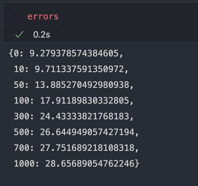
Intuitively we can see that plots for λ = 0 and λ = 10 are quite good, just to be sure we stored the root mean squared error in a dictionary errors let's print it out and see which λ got the least error.

We can see that λ = 0 got the least error and λ = 10 is slightly greater than that but just be on the safer side we will pick λ = 10 for our hypothesis.
Great work everyone, we have successfully learnt and implemented our first machine learning algorithm of Linear Regression using a Normal equation on 2 datasets. There are a few things that we need to keep in our mind while using the Normal equation method. This method is not efficient with respect to computation time on large datasets (samples > 10,000) and the reason is the operation of calculating the inverse of a matrix that had a time complexity of around O(n3).
So in that case Gradient Descent method comes very handy and we'll be going to learn that in our next article. Also, we'll be exploring Regularization in great depth too.
I hope you have learnt something new, for more updates on upcoming articles get connected with me through Twitter and stay tuned for more. Till then enjoy your day and keep learning.
22

