22
Pandas Skills Pt. 1 🐼📊📚📐
Before all, here is the link with the code of this lecture.

The most fundamental aspect of Pandas, is the DataFrame.
This is how your data is stored, and it's a tabular format with rows and columns as you'd find them in a spresheet or a relational database table. So, before I dive into some more advanced Pandas topics, let me review the DataFrame concept.
import pandas as pdAfter importing Pandas as 'pd', I'm going to create a Dictionary called 'scores'. A dictionary, is a Python structure which stores key-value pairs. In this dictionary the keys are 'name', 'city' and 'score', and the values are lists, as denoted by the square brackets, which are mapped to their corresponding key.
scores = {'name':['Hugo,', 'David', 'René'],
          'city':['Guatemala', 'Estanzuela', 'Zacapa'],
            'score':[50,70,100]}
Now, I'm going to transform this dictionary, into a Pandas DataFrame.
df = pd.DataFrame(scores)To see the data, just type the name of the DataFrame.
dfAnd you should see a table with 'name', 'city' and 'scores' as column headers. And three rows of corresponding data.
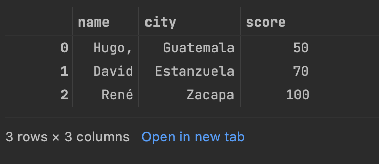
Each columns is a series, and notice the values zero, one, and two to the left. These are the Index of our DataFrame. And are useful for referencing and subsetting our
data.
If we wanted to just return one column in our Data Frame, the notation is the DataFrame, and then the column name or names in square brackets. Let's take a look at 'score'.
df['score']
You can also call df.score to return the same result.

Similarly, you can also create new columns in your DataFrame by passing a new column name into the square brackets and assigning it.
Here, I'm creating a new column that combines the 'name' and 'city' columns.
df['name_city'] = df['name'] + '_' + df['city']Now let's say I wanted to subset my data to only show those folks with scores above, say 70. To do that, I can create a boolean expression which returns true for scores greater than 70, and only return those records where this condition is true.
df[df['score']>69]
Pandas is very flexible, in that you can import data, from a wide variety of data sources, including CSV's, Excel files, JSON files, databases, Parquet files, you name it.
I'm going to import the Iris dataset, as a DataFrame called 'iris'. This is a common sample dataset for practicing Datascience.
You can find the link of the dataset from Kaggle, here.
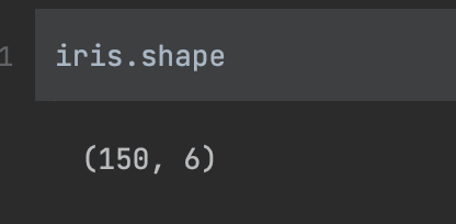
iris = pd.read_csv('iris.csv')DataFrames have an attribute called 'shape', which tell us the dimensionality of our data. By calling the name of the data frame, followed by the '.shape' I can see the number of rows and columns that the data frame has.
To preview the data, there's the 'head' function will return the top records of the DataFrame.

Similarly, I can see the bottom rows with the 'tail' function.

Working with data in Pandas, datatypes are very important and will influence what operations can be performed. I found Pandas to be pretty intelligent in how it assigns datatypes, but as the Russians say: "trust, but double check".
To do this, call the dtypes attribute on your data
frames.

There are two datatypes represented in this DataFrame, float for all the measurement data, and object for the species.
Often when using pandas, you'll want to subset your data, and 'loc' allows you to subset your data based on index labels, so either the row indexes or column names, 'iloc' subsets by position, so the row number or column order.
I'm going to subset this DataFrame based on row indexes three, four and five, which are the fourth through sixth rows of our data. Note indexing begins at zero.

We can also return a single-cell value, by passing a row and column names separated by a comma.
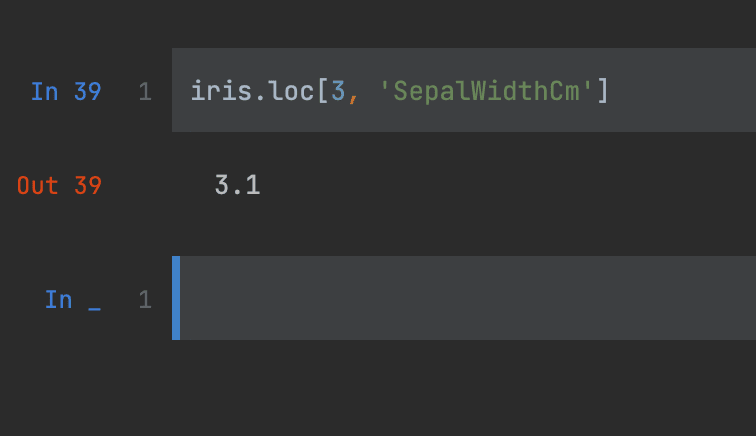
This returns 3.1, which is the measurement for sepal length for the row at index three in our data frame.
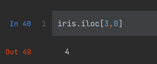
Using 'iloc' I can return the same value by referencing the same row index of three but a column index of zero.
Often, after you've done a whole host of data transformation with Pandas, you want to export your DataFrame for analysis or visualization.
A handy way to do this is the 'to_csv' function.
iris.to_csv ('iris-output.csv', index=False)Note you may want to include index equal to false, so the index isn't included in your CSV.
Pandas has an option system, which allows you to customize how the package works for you. Most often, this can be useful to change how results are displayed in Pandas. Here's an example.
import pandas as pd

emissions = pd.DataFrame \
({"country": ['China', 'United States', 'India'],\
"year": ['2018', '2018', '2018'],\
"co2 emissions": [10060000000.0,5410000000.0,2650000000.0]})

emissions
I will start with this simple DataFrame, the first option which comes in handy is to configure the maximum row size display for a Pandas DataFrame.
If we set the max row size to two, here's what we get.
pd.set_option('max_rows', 2)
emissions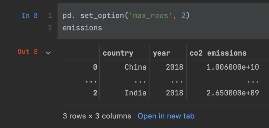
So you see two rows displayed, separated by an ellipses, that's what this option does.You can either use it to limit the screen space your displayed data frames take up or conversely to expand the row size, to reveal more of your data. Similarly, the max columns display option will
reveal or hide columns. I find this most useful when viewing the head of a data frame that has a lot of columns as Pandas will truncate these by default.

By modifying the float format option, you can display values with a lots of decimals, normally, and even add in a comma as 1,000 separator.
pd.options.display.float_format = '{:,.2f}'. format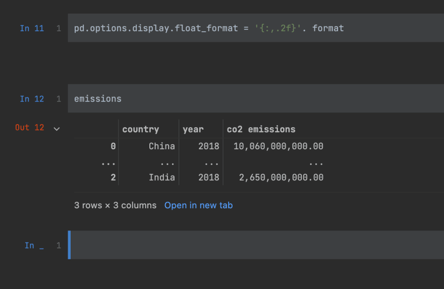
One area where you might encounter some hurdles with pandas is dealing with data types. As I said at the beginning of this article, Pandas, generally speaking it's pretty good at assigning proper data types nonetheless, you'll find many instances when you need to convert data types.
To give you a couple of examples, I'm going to leverage the planets dataset, as it has a good variety of data types.
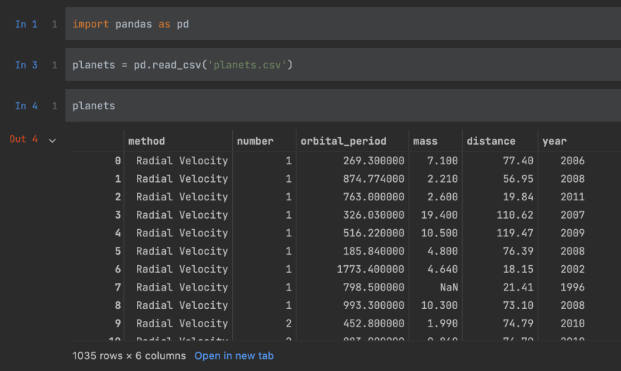
From looking over the data frame, you can probably infer what the data type assignments will be, but to be sure I can access the types attribute of planets.
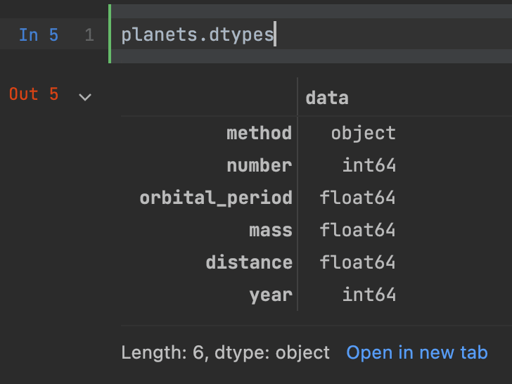
Now, the data types varying from an object to integers to floats. How pandas handles your data depends on the data types you've designated. For example, If I use the 'mean' function to return the average for all float and integers in the dataset.

Aside from some warning, everything looks OK, but you might question whether it really makes sense to take an average of the year as I've done here.
Let's see how different data types interact.
Here, I'm dividing an integer column by a float.
planets['number'][0]/planets ['mass'][0]The result is a float, great, that's what you'd hope
for.

I also have the ability to change data types using the 'astype' function. For instance, I can convert the integer value of the 'number' column to a float.
planets['number'][0].astype(float)
It's useful to see what happens when you convert a float to an int.

In this case, we've lost the decimal point. And it's worth noting that this approach would effectively round down any floats as you convert to integers.
I can also cover the 'year' to an object by calling the 'astype(str)' for string.
planets['year'][0].astype(str)
To take advantage of the date time data type in Pandas I can convert the integer 'year' value to a date time using 'to_datetime' and then specify how the data is currently
formatted.
planets['year_dt'] = pd.to_datetime(planets['year'], format='%Y')
planets['year_dt']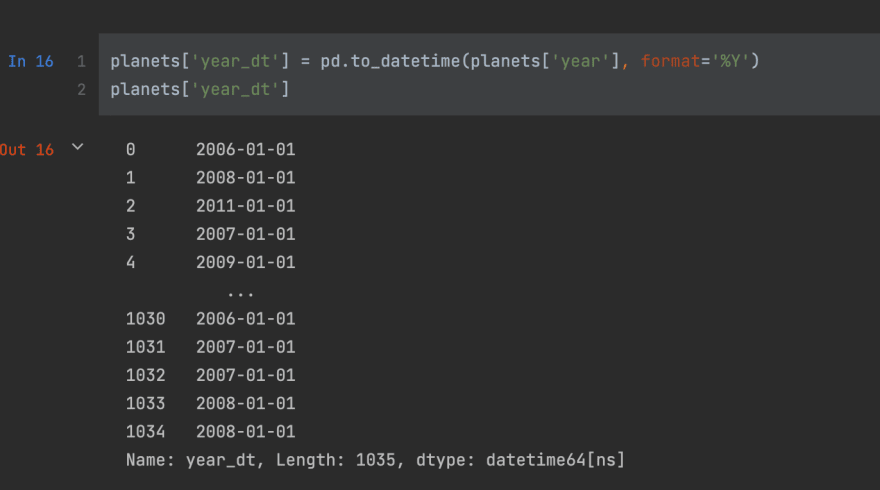
22
