
25
Walmart Store Sales Forecasting
The objective of this project is to:
We will import necessary packages as follows:
import numpy as np
import pandas as pd
import matplotlib.pyplot as plt
import seaborn as sns
import plotly.express as px
%matplotlib inlineThe dataset contain the following files in the csv format:
train.csv : this file has 421570 rows and 5 columns. The columns contain the information for a store, department, date, weekly sales and whether a particular week is a holiday week or not
store.csv : this file has 45 rows and 3 columns. The columns correpond to the stores, their type and sizes of stores
features.csv : this file 8190 rows and 12 columns. This file again has some further information regarding the stores and the region in which a particular store is located. It has date, temperature, fuel price, consumer price index, unemployment rate information for the region in which a particular store is located. It also has 5 columns MarkDown1-5 which corresponds to some promotional activities going on in different stores.
walmart = pd.read_csv('train.csv')
stores = pd.read_csv('stores.csv')
features = pd.read_csv('features.csv')
testing = pd.read_csv('test.csv')
Merging of Data
Let's merge the data from 3 dataframes into a single dataframe and proceed further with a one dataframe.
Let's merge the data from 3 dataframes into a single dataframe and proceed further with a one dataframe.
merged = walmart.merge(stores, how='left').merge(features, how='left')
testing_merged = testing.merge(stores, how='left').merge(features, how='left')
Extracting Date Information
The sales are given for Years 2012-2012 on weekly basis. So let's split the date column to extract information for year, month and week
def split_date(df):
    df['Date'] = pd.to_datetime(df['Date'])
    df['Year'] = df.Date.dt.year
    df['Month'] = df.Date.dt.month
    df['Day'] = df.Date.dt.day
    df['WeekOfYear'] = (df.Date.dt.isocalendar().week)*1.0

split_date(merged)
split_date(testing_merged)
Columns Information: Data Types
merged.info()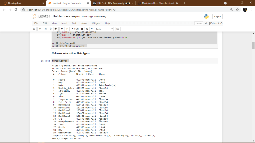
Missing Values
missing_values = merged.isna().sum()
px.bar(missing_values,
       x=missing_values.index,
       y=missing_values.values,
       title="Missing Values",
       labels=dict(x="Variable", y="Missing Values"))
From the above plot;
Markdown1-5 contain lots of missing values, more than 250000 in each markdown column.
Markdown1-5 contain lots of missing values, more than 250000 in each markdown column.
Popularity of Store Types

Insights;
Type A stores are more popular than the B and C types
Insights;
Type A stores are more popular than the B and C types
Average Monthly Sales - Per Year
Insights
Month of January witnessed the lowest sales for 2011 and 2012 while for 2010 the weekly sales are not given in the data.
From Feburary till October the weekly sales nearly remains constant around 15000 for the 3 years.
November and December showed the highest sales for 2010 and 2011 while for 2012 the sales data has not been provided.
As shown below;

Average Weekly Sales - per Year
Insights
Insights
As shown;

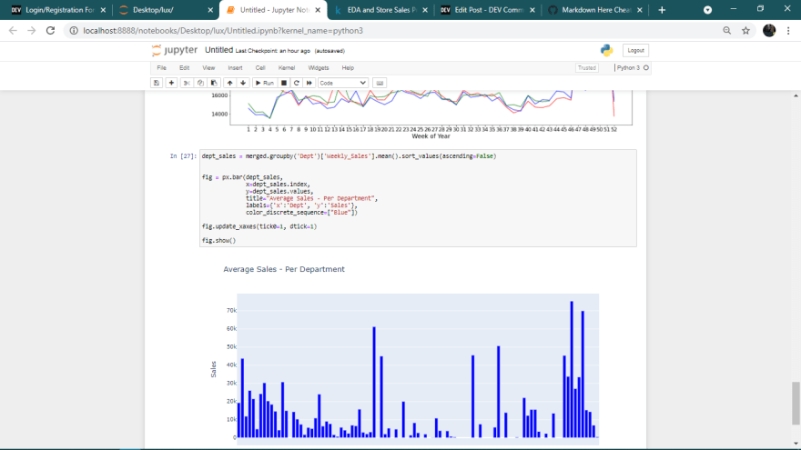
Average Department Sales
Different departments showed different levels of average sales
As shown;
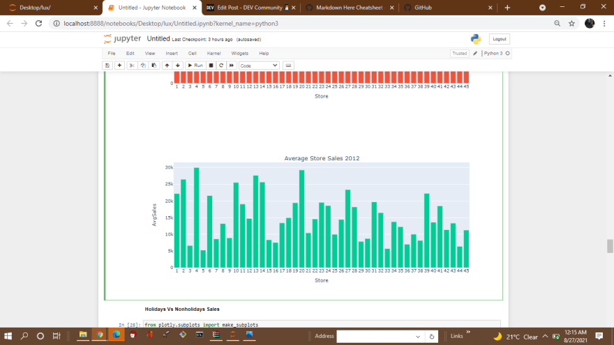
Average Store Sales - Year Wise


Holidays Vs Nonholidays Sales
*Despite being the less percentage of holiday weeks the sales in the holidays week are on the average higher than in the non-holiday weeks.
*Despite being the less percentage of holiday weeks the sales in the holidays week are on the average higher than in the non-holiday weeks.

Relationship: Week of Year vs Sales
Weekly sales increases towards the end of the year as shown;

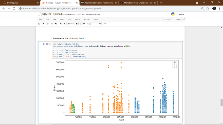
Relationship: Size of Store vs Sales
Relationship: Fuel Price vs Sales

Relationship: Unemployment vs Sales

Correlation Matrix
Lets now study the relationship between the different columns numerically to check how they correlate with the weekly sales in order to confirm the inferences we have gathered from the above EDA study.
To carry out Correlation Matrix we will first convert the 'Type' column to numerical values as shown;
storetype_values = {'A':3, 'B':2, 'C':1}
merged['Type_Numeric'] = merged.Type.map(storetype_values)
testing_merged['Type_Numeric'] = testing_merged.Type.map(storetype_values)
Insights obtained from above correlation matrix are;
Following steps will be performed for preparing the data for the subsequent model training.
merged = merged.drop(['Date', 'Temperature','Fuel_Price', 'Type', 'MarkDown1', 'MarkDown2', 'MarkDown3',
             'MarkDown4', 'MarkDown5', 'CPI', 'Unemployment', 'Month', 'Day' ], axis=1)

testing_merged = testing_merged.drop(['Date', 'Temperature','Fuel_Price', 'Type', 'MarkDown1', 'MarkDown2', 'MarkDown3',
             'MarkDown4', 'MarkDown5', 'CPI', 'Unemployment', 'Month', 'Day' ], axis=1)
Identify input and target columns.
input_cols = merged.columns.to_list()
input_cols.remove('Weekly_Sales')
target_col = 'Weekly_Sales'

X = merged[input_cols].copy()
y = merged[target_col].copy()
Scale the values
from sklearn.preprocessing import MinMaxScaler

scaler = MinMaxScaler().fit(merged[input_cols])

X[input_cols] = scaler.transform(X[input_cols])
testing_merged[input_cols] = scaler.transform(testing_merged[input_cols])
Create training and testing sets
from sklearn.model_selection import train_test_split
X_train, X_test, y_train, y_test = train_test_split(
X, y, test_size=0.3, random_state=42)We will use Linear regression algorithm.
from sklearn.linear_model import LinearRegression

# Create and train the model
model = LinearRegression()
model.fit(X,y)

# Generate predictions on training data
train_preds = model.predict(X_train)
train_preds
Output will be;
array([17035.12035741, 15737.5350701 , 22990.63793901, ...,
       20276.77727003, 21110.53004444, 23548.55581834])
25