
31
Activation Functions used in Neural network with Advantages and Disadvantages
Deep learning needs lots of data to perform efficiently. Today internet provides tons of data but the issue with it is that there is no solid partition between the useful and not-so-useful data. In technical terms, there is some amount of noise without out required information. If we train our learning model without removing the noise, our model will not produce the required output. This is where the Activation Function comes into the picture.
Activation functions are mathematical equations that determine the output of a neural network model. They help the network to use the important information and suppress the noise.
In a neural network, activation functions are utilized to bring non-linearities into the decision border. The goal of introducing nonlinearities in data is to simulate a real-world situation. Almost much of the data we deal with in real life is nonlinear. This is what makes neural networks so effective.
Before we dive deeper into different types of activation functions, let's first look at where is activation function used in a neural network.
Following is the picture of a simple model of neuron commonly known as the perceptron. It can be divided into 3 parts: Input layer, neuron, and output layer.

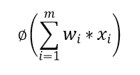
We have input as X1, X2, X3,..., Xm. and the weights associated with those inputs as w1, w2, w3,...,wm.
We first calculate the weighted sum of the input i.e.

Then Activation function is applied as,
The calculated value is then passed to the next layer if present.
Now let's look at the most common types of Activation functions used in deep learning. We will also learn how to implement using python.
Sigmoid Activation Function is one of the widely used activation functions in deep learning. As its name suggests the curve of the sigmoid function is S-shaped.
Sigmoid transforms the values between the range 0 and 1.
The Mathematical function of the sigmoid function is:

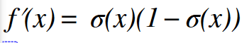
Derivative of the sigmoid is:
Python Code
import numpy as np
import matplotlib.pyplot as plt

# Sigmoid Activation Function
def sigmoid(x):
  return 1/(1+np.exp(-x))

# Derivative of Sigmoid
def der_sigmoid(x):
  return sigmoid(x) * (1- sigmoid(x))

# Generating data to plot
x_data = np.linspace(-10,10,100)
y_data = sigmoid(x_data)
dy_data = der_sigmoid(x_data)

# Plotting
plt.plot(x_data, y_data, x_data, dy_data)
plt.title('Sigmoid Activation Function & Derivative')
plt.legend(['sigmoid','der_sigmoid'])
plt.grid()
plt.show()

Advantages:
- The output value is between 0 and 1.
- The prediction is simple, ie based on a threshold probability value.
Disadvantages:
- Computationally expensive
- Outputs not zero centered
- Vanishing gradient—for very high or very low values of X, there is almost no change to the prediction, causing a vanishing gradient problem. This can result in the network refusing to learn further, or being too slow to reach an accurate prediction.
The tanh function is similar to the sigmoid function. The output ranges from -1 to 1.
The Mathematical function of tanh function is:

Derivative of tanh function is:

Python Code
import numpy as np
import matplotlib.pyplot as plt

# Hyperbolic Tangent (htan) Activation Function
def htan(x):
  return (np.exp(x) - np.exp(-x))/(np.exp(x) + np.exp(-x))

# htan derivative
def der_htan(x):
  return 1 - htan(x) * htan(x)

# Generating data for Graph
x_data = np.linspace(-6,6,100)
y_data = htan(x_data)
dy_data = der_htan(x_data)

# Graph
plt.plot(x_data, y_data, x_data, dy_data)
plt.title('htan Activation Function & Derivative')
plt.legend(['htan','der_htan'])
plt.grid()
plt.show()

Advantages:
- Zero Centered
- The prediction is simple, ie based on a threshold probability value.
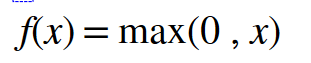
The rectified linear activation function (RELU) is a piecewise linear function that, if the input is positive say x, the output will be x. otherwise, it outputs zero.
The mathematical representation of ReLU function is,
The derivative of ReLU is,

ReLU is used widely nowadays, but it has some problems. let's say if we have input less than 0, then it outputs zero, and the neural network can't continue the backpropagation algorithm. This problem is commonly known as Dying ReLU. To get rid of this problem we use an improvised version of ReLU, called Leaky ReLU.
Python Code
import numpy as np
import matplotlib.pyplot as plt

# Rectified Linear Unit (ReLU)
def ReLU(x):
  data = [max(0,value) for value in x]
  return np.array(data, dtype=float)

# Derivative for ReLU
def der_ReLU(x):
  data = [1 if value>0 else 0 for value in x]
  return np.array(data, dtype=float)

# Generating data for Graph
x_data = np.linspace(-10,10,100)
y_data = ReLU(x_data)
dy_data = der_ReLU(x_data)

# Graph
plt.plot(x_data, y_data, x_data, dy_data)
plt.title('ReLU Activation Function & Derivative')
plt.legend(['ReLU','der_ReLU'])
plt.grid()
plt.show()

Advantages:
- Non-Linear
- Computationally efficient
Disadvantages:
- Dying ReLU problem i.e for the inputs 0 or negative the gradient of ReLu becomes zero and thus the network cannot make backpropagation.
Leaky ReLU is the most common and effective method to solve a dying ReLU problem. It is nothing but an improved version of the ReLU function. It adds a slight slope in the negative range to prevent the dying ReLU issue.
The mathematical representation of Leakt ReLU is,

The Derivative of Leaky ReLU is,
Python Code
import numpy as np
import matplotlib.pyplot as plt

# Leaky Rectified Linear Unit (leaky ReLU) Activation Function
def leaky_ReLU(x):
  data = [max(0.05*value,value) for value in x]
  return np.array(data, dtype=float)

# Derivative for leaky ReLU
def der_leaky_ReLU(x):
  data = [1 if value>0 else 0.05 for value in x]
  return np.array(data, dtype=float)

# Generating data For Graph
x_data = np.linspace(-10,10,100)
y_data = leaky_ReLU(x_data)
dy_data = der_leaky_ReLU(x_data)

# Graph
plt.plot(x_data, y_data, x_data, dy_data)
plt.title('leaky ReLU Activation Function & Derivative')
plt.legend(['leaky_ReLU','der_leaky_ReLU'])
plt.grid()
plt.show()

Advantages:
- modification of the ReLU function to solve the dying ReLU problem.
Disadvantages:
- leaky ReLU does not provide consistent predictions for negative input values.
31