
34
Beginner EDA on Video Game Sales - Kaggle Dataset
Data Science has become a booming field recent couple of years. It is the most hot topic right now besides AI/ML and Deep Learning. Since, the data is in abundance and the Big Companies need to get to know their crowd for maximizing their profits, Data Analysis and Data Science concepts are applied.
In any ML project, the steps are followed like this:
1] Data Collection
2] EDA
3] Feature Engineering
4] Feature Selection
5] Outlier
6] Model Creation
7 Deployment
I am here to talk about the EDA that I have done in the Video Game Sales data set in Kaggle.
Exploratory Data Analysis is the most crucial part of the Data Science project. It can "Make Or Break" your project as most of the important insights as well as predictions can be done using EDA concepts.
I have applied Concepts of EDA on Video Game Sales Data set of Kaggle.
Here's the link to my Kaggle Notebook:
Basic EDA on Video Game Sales - Kaggle
Here's the link to my Kaggle Notebook:
Basic EDA on Video Game Sales - Kaggle
Always we need to know what our data set is and what all libraries the project needs.
There are 16,598 records. 2 records were dropped due to incomplete information.
There are 16,598 records. 2 records were dropped due to incomplete information.
It contains around
The video Game Sales data includes 11 fields/columns. They are:
The video Game Sales data includes 11 fields/columns. They are:
So, we import the libraries:
import numpy as np # linear algebra
import pandas as pd # data processing, CSV file I/O (e.g. pd.read_csv)
import matplotlib.pyplot as plt # for data visualization
%matplotlib inline
import seaborn as sns # for advanced data visualizations
After importing the libraries, we import the data set:
vgSales = pd.read_csv("../input/videogamesales/vgsales.csv")
vgSales.head()
Here, the data file was a .csv file i.e. a comma separated value file.
VariableName = pd.read_csv("file_name.csv")Comma Separated Values means that, the values in the file or records is separated by comma i.e. ','.
Here, to see the first 5 records of the data frame we have created using Pandas Library, I have used .head() function.
Now after importing the data set successfully, we are ready to go for the data cleaning.
Here, to see the first 5 records of the data frame we have created using Pandas Library, I have used .head() function.
Now after importing the data set successfully, we are ready to go for the data cleaning.
To get information from the data about its column names, its data types, Null Count etc., we use .info() and .isna().sum():
vgSales.info()
vgSales.isna().sum()
We can observe that the Year column is having 271 NA records and the Publisher column is having 58 NA records, which makes a total of 329 NA records in the data set.
Hence, we need to remove these before visualization and taking useful insights from them.
Hence, we need to remove these before visualization and taking useful insights from them.
Apart from the NA values worrying us, we can also find the other anomalies present in the data set.
This data set holds records till 2017th Year. But when we try to find the maximum value of the records in Year column, I get a crucial anomaly.
print("Max Year Value: ", vgSales['Year'].max())By this function code we can get the max value in the column we want. This showed that the Year column had maximum value 2020. Then I mined out that record to investigate carefully.
maxEntry = vgSales['Year'].idxmax()
vgSales.iloc[maxEntry]
I observed that it gave a game record that wasn't released in 2020 Year but it was actually published by Ubisoft on 2009. This was the output.

I then replaced the value with the correct one.
vgSales["Year"] = vgSales["Year"].replace(2020.0, 2009.0)
print("Max Year Value: ", vgSales["Year"].max())
Now, this was just one anomaly. I found out that there were many anomalies like these. So, decided to replace them with the year 2009 as the visualization of that data showed that 2009 was the year in which most of the games were produced or released.
YearAnamoly = vgSales[vgSales['Year'].isnull()]['Name'].unique()
print("The year records having such anomaly: ", len(YearAnamoly))
There were 233 such records.
plt.figure(figsize = (20,20))
plt.bar(vgSales["Year"].value_counts().index, vgSales["Year"].value_counts())
plt.title("The most games produced in a specific year")
plt.show()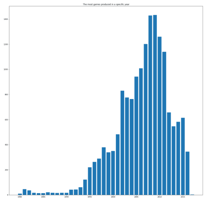
vgSales['Year'] = vgSales['Year'].fillna(2009.0)
vgSales['Year'].isnull().sum()
After this all the NA values were eradicated from Year column. I then converted the Year column Data Type which was float64 to int64 like this:
vgSales['Year'] = vgSales['Year'].astype('int64')I then removed the 58 NA Records in Publisher because it won't affect the visualization as it was an unnecessary noise in the data using .dropna() function.
After anomalies and NA record cleaning I thought of removing the Skewness of columns that are numeric like NA_Sales, EU_Sales, JP_Sales, Other_Sales, Global_Sales etc.
print("The Skew Count of NA_Sales Column is:",vgSales["NA_Sales"].skew())
print("The Skew Count of EU_Sales Column is:",vgSales["EU_Sales"].skew())
print("The Skew Count of JP_Sales Column is:",vgSales["JP_Sales"].skew())
print("The Skew Count of Other_Sales Column is:",vgSales["Other_Sales"].skew())
vgSales["NA_Sales"] = vgSales["NA_Sales"]**(1/2)
vgSales["EU_Sales"] = vgSales["EU_Sales"]**(1/2)
vgSales["JP_Sales"] = vgSales["JP_Sales"]**(1/2)
vgSales["Other_Sales"] = vgSales["Other_Sales"]**(1/2)
vgSales["Global_Sales"] = vgSales["NA_Sales"] + vgSales["EU_Sales"] + vgSales["JP_Sales"] + vgSales["Other_Sales"]
Now, the cleaning and normalization of data was over and Exploratory Data Analysis and Visualization started.
vgSales[["Genre","Global_Sales"]].groupby("Genre").sum()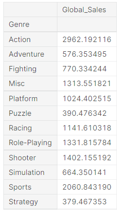
plt.figure(figsize = (20,20))
plt.bar(vgSales["Platform"].value_counts().index, vgSales["Platform"].value_counts())
plt.title("Most Games produced in Specific Gaming Platform")
plt.show()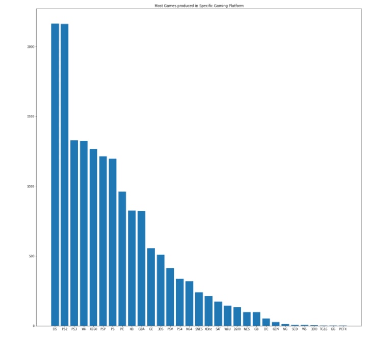
We can see that DS and PS2 are tied for the top spot in this.
With this, I did the basic EDA of this data set.
Here is my Linkedin Profile:
Siddhesh Shankar
Here is my github repo link:
SiddheshCodeMaster
Here is my Linkedin Profile:
Siddhesh Shankar
Here is my github repo link:
SiddheshCodeMaster
Happy Data Cleaning ! Happy Exploration ! Happy Learning !
34