21
A look into Dynamic Programming - Matrix Chain Multiplication
In the beginning of the last article I wrote, I described two ways of solving a problem by splitting it into subproblems: on one hand, those problems can be solved independently from one another (a method called divide & conquer, which I described in the article); on the other hand, they can interact with each other, building up on the results. Problems on the latter category can be solved using a method called dynamic programming, which will be the topic for today.
In the field of Computer Science, Dynamic Programming is derived from a mathematical optimisation method. It refers to simplifying a problem by breaking it down into smaller subproblems. If the results of those smaller subproblems overlap so they can be fit inside the larger problems, then there is a relation between them and the results of the larger problem.
For example, by modifying the BFS algorithm I presented in this article to find the shortest path in an unweighted graph we can obtain a dynamic programming solution to the problem.
This is possible by making a simple statement: if i and j are two nodes in an unweighted graph, then the shortest path from i to j would be obtained by first obtaining the shortest path from i to a neighbour of j. Described in pseudocode:
min_dist[i][j] = infinity
for every neighbour k of j:
   min_dist[i][j] = min(min_dist[i][k]+1, min_dist[i][j])
The last line of the snippet is called a reccurence relation. (such relations are widely used in mathematics; another example is the way the Fibonacci sequence is calculated.
Subproblems are basically smaller instances (or versions) of the original problem. By saying that a problem has "overlapping subproblems", we mean that finding its solution involves solving the same subproblem multiple times.
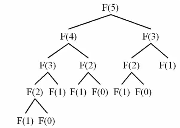
An accessible example is calculating the n-th Fibonacci number, which I presented in an earlier article. Let's look again at the recursion tree of the problem:

It is clear that, if we do not store the results in some way, some numbers will be calculated multiple times, resulting in a staggering time complexity of O(1.62^n) (see the article for information about how this was calculated).
This technique is called "memoization" - we can store the value of a Fibonacci number in an array after we calculate it for later use. This would decrease the time complexity, in this case, to an ~O(n).
Memoization is widely used in dynamic programming (which is, in essence, an optimisation technique). Let us see how we can create such a solution.
We know that matrix multiplication is not a commutative operation, but it is associative. It also turns out that the order in which the multiplication is done affects the overall number of operations you do.
Let's suppose we have three matrixes:
- A, of size 3 x 1 - a column matrix
- B, of size 1 x 3 - a line matrix
- C, of size 3 x 1 - a column matrix again
We can multiply them in two ways:
- (AB)C - multiplying A and B would yield a 3 x 3 matrix, and would take 9 operations. Multiplying (AB) with C would take another 9 operations, for a total of 18 operations.
- A(BC) - multiply B and C only takes 3 operations and yield a 1 x 1 matrix. Multiplying A with (BC) would take another 3 operations, for a total of 6 operations.
Keeping that in mind, we ask the question: what is the best order to do the multiplication?
Let's suppose we have N matrixes (M_1 through M_N) whose sizes we store in an array S, such that S[i-1] and S[i] are the sizes for matrix i.
We can solve the problem using dynamic programming by making the following observation: the first thing we need to determine is what multiplication should be done last. In other word, we search for a matrix i such that our expression would look like (M_1 * M_2 * ... M_i ) * ( M_(i+1) * ... M_N), and both the products in parenthesis are also calculated optimally.
We can construct an N x N 2D array, let's call it A, such that A[i][j] will hold the minimum cost (number of operations) to compute the product of matrixes from M_i through M_j. We will use this array to memoise the results.
Let's see how we can calculate the cost for a "cut" in the product of matrixes from M_i through M_j. If we were to put the parenthesis such like (M_i * M_(i+1) * .... M_k) * (M_(k+1) * ... M_j), the cost would be the sum of the cost of the two parenthesis + the cost to multiply the matrix yield by those two, which will be S[i-1] * S[k] * S[j], as the first result would be of size S[i-1] x S[k], and the second would be of size S[k] * S[j].
We now just have to find the best k for our cut. We can make this in a recursive manner. Let us look at an implementation of the idea:
The sizes for the matrixes is the one in the example above, rows and column matrixes. The code outputs the result as 6, as we have concluded earlier.
This was achieved recursively, by first calling matrix_chain_cost for positions 1 through N. We used memoisation to avoid redundant calculations, and then applied the formula we found above.
The time complexity of the code above is O(n^3), as we are basically generating the cost for all the "cuts" we can do in the expression.
That was all for today. The Magic of Computing will be back with yet another interesting algorithmic topic. But, until then, maybe you fancy some Graph Theory? Or are you more of a Backtracking person?
21
