IRIS Dataset Implementation

Introduction

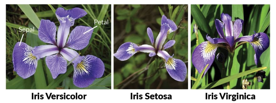
IRIS DataSet consists of 150 rows and 5 columns where the columns are namely sepal length in cm, sepal width in cm, petal length in cm, petal width in cm, and Species. There are 3 species namely Iris Setosa, Iris Versicolor, and Iris Virginica.

Dataset can be accessed through this Link.

Another feature of this dataset is it has the right proportion of data for each species. Meaning it has 50 rows of data for each Species. Also, this dataset is very clean and hence liked by most beginners to start with ML.

These are the 3 different species of the IRIS Dataset pictorially.

Now let's get our hands dirty by coding. For which you require Google Colab, Visual Studio Code (or any IDE), Dataset (downloaded from the above link in the form of CSV), and excitement to learn something.

Framing the Problem

Our ultimate goal is to describe the Species to which the flower belongs provided length and width of sepal and petal.

Data Preprocessing and Visualization

Importing Necessary Libraries
Initially let us import all the necessary libraries that are required to run the code.

import numpy as np
import pandas as pd

import seaborn as sns

from sklearn.model_selection import train_test_split
from sklearn.linear_model import LogisticRegression

Here we import NumPy, Pandas, Matplotlib, Seaborn, and other necessary modules from Sklearn.

After importing the necessary libraries let's import the IRIS Dataset that we are going to work on.

Importing Dataset

To import, we have to use the pandas library which has the 'read_csv' function which takes the file path to import the necessary dataset.

data  = pd.read_csv('iris_data.csv')
data

After importing if we print the data we find that there are 150 rows and 5 columns. Further, if we dig deeper we find no null values, meaning all the rows and columns are filled and reduce the huge burden. After that I have encoded (to change into a form that is better usable) the Species as follows:

Iris Setosa
Iris Virginica
Iris Virginica

The code for the same is given below:

onehot = []

for i in data['Species']:
    if (i == 'setosa'):
        onehot.append(1)
    elif (i == 'virginica'):
        onehot.append(3)
    else:
        onehot.append(2)
data['Species'] = onehot

Visualizations

I have implemented it understandably but it could be implemented in many ways at your convenience. Then now it's time to visualize the data using Matplotlib and Seaborn.

Using the 'countplot' function I have plotted the count of each Species which is found to be 50 each (same as the statement mentioned at the beginning). Code to implement the same is:

sns.countplot(data['Species'])
plt.show()

Now there is something called a FacetGrid plot where we can plot dataset onto multiple axes arrayed in a grid of rows and columns that corresponds to levels in the dataset. Code to implement the same is:

sns.FacetGrid(data, hue ="Species",height = 6).map(plt.scatter, 'Sepal.Length', 'Petal.Length').add_legend()
plt.show()

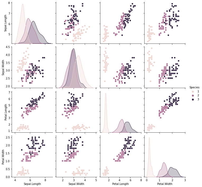
There is one more interesting plot called a "pairplot" where we plot many scatter plots with the data available in the total number of numerical columns. For better understanding let's consider our dataset which has 4 numerical columns. So there would be 4 * 4 possible scatter plots available. Sounds interesting right it will look even better while we visualize it.

Code to implement the same (small code, big difference):

sns.pairplot(data, hue="Species")
plt.show()

Hope it's understandable after visualizing it though it looks messy while understanding it. Now it's time to build our model. Now let's move on to the model building.

Model Building:

It is considered one of the most important parts of any ML Workflow. I have addressed in this blog one classification algorithm i.e. Logistic Regression. But the code contains its implementation using KNN and Decision Tree Classifier as well.

Before directly building the model we have to separate the independent and dependent variables. In our case, the Independent variables are columns Length and Width of Sepal and Width. We can easily separate it using the "iloc" function.

X = data.iloc[ : , : 4]
y = pd.DataFrame(data['Species'])

Now we have to split the data for Training and Testing. Now a doubt arise in what ratio are we supposed to split to get optimal results. It's actually a trial and error method but most often it is preferred to have a 70:30 or 75:25 split as they work in most cases. In our case, I have used a 75:25. There is no hard and fast rule. You can try different split sizes and get better results as well.

X_train, X_test, y_train, y_test = train_test_split(X, y, test_size = 0.25, random_state = 0)

After successfully splitting the train and test data we have to fit the train data on the Logistic Regression model.

model = LogisticRegression()
model.fit(X_train, y_train)

Hurrah!! The model has been successfully trained now we have to actually test the working of the model where I provide some random values as input and predict the output provided by the model.

X_new = np.array([[5, 2.9, 1, 0.2]])
print("X_new.shape: {}".format(X_new.shape))

If you feel that the output for the set of input values provided is perfect then Congratulations on that note, you have successfully build your model. Now we come to the end of this blog and I hope it was very much useful and has given clear insights on how to process with the IRIS Dataset.

This is the GitHubLink for the code used in the blog.

Please feel to post your views and comments on how to improve and if I have had some Typos in the Blog as well.

Feel free to connect with me through LinkedIn.

Happy Learning and Blogging!!!

HackThisFall 2.0

Hey folks,

I am thrilled to inform you that I have been accepted as a “Hackathon Evangelist” for Hack This Fall 2.0!🎉

Super excited to bring a change and contribute to the hacker community in a meaningful way!🚀

Do Register for Hack This Fall 2.0 here🔗:

Register in the hackathon by heading over to the link given above and enter the special code "HTFHE067" to earn some exclusive participation goodies along!!