20
Intro to Machine Learning
Welcome to my third blog!
In this blog, I am revising basic concepts in the Kaggle course (Intro to machine learning) and we'll build our very first model here and it's totally basic so, it doesn't require any experience in this topic, Let's start!
Lesson 1 : How models work?
Let's walk through the example there:
- Your cousin has made millions of dollars speculating on real estate. He's offered to become business partners with you because of your interest in data science. He'll supply the money, and you'll supply models that predict how much various houses are worth.
When you wondered how he predicted the house prices before he said by "intuition", But more questioning reveals that he's identified price patterns from houses he has seen in the past and he uses those patterns to make predictions for new houses he is considering.
Machine learning works the same way. We'll start with a model called the Decision Tree. There are fancier models that give more accurate predictions.

What is that?
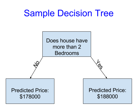
- The DT (decision tree) divides houses into only two categories.
- We use data to decide how to break the houses into two groups
- Then again to determine the predicted price in each group. This step of capturing patterns from data is called fitting or training the model.
- After data has been fit, you can apply it to new data to predict prices of additional new homes.
Improving the Decision Tree

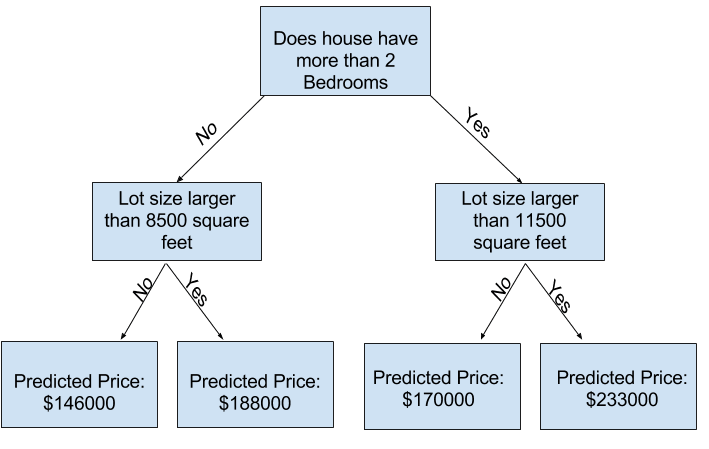
Now, It pops up in your mind that definitely DT 1 makes more sense as when the more no. of bedrooms the higher price it'll be, right?
Well, This not totally true.
As there are extra features (e.g. lot size, crime rate and so on).
This will lead us to the deeper tree that covers more features that definitely affects the predicted price and those are the extra "splits".

leaf is where we have our predicted price.
The splits and values at the leaves will be determined by the data, so we need to check out the data we'll be working with.
Lesson 2 : Basic Data Exploration (Examine your data)
To build any ML model we need to be familiar and fully understand our data, In order to do so, One of the well known libraries is "Pandas".
What's pandas?
Pandas is the primary tool used for exploring and manipulating data.
Pandas => pd
Let's import it :
import pandas as pdThe most important part of the Pandas is the "DataFrame".
A DataFrame holds the type of data you might think of as a table. This is similar to a sheet in Excel, or a table in a SQL database.
Pandas has powerful methods for most things we'll want to do with this type of data.
Let's do some code!
Check this dataset : Homes in Melbourne, Australia
As usual, Check my code
Interpreting Data Description
The results show 8 numbers for each column in our original dataset. The first number is count that shows how many rows have non-missing values.
Missing values arise for many reasons. For example, the size of the 2nd bedroom wouldn't be collected when surveying a 1 bedroom house. We'll come back to the topic of missing data.
The second value is the mean, which is the average.
The third value is std (standard deviation) which measures how numerically spread out the values are.
To interpret the min, 25%, 50%, 75% and max values, imagine sorting each column from lowest to highest value.
The first (smallest) value is the min.
If you go a quarter way through the list, you'll find a number that is bigger than 25% of the values and smaller than 75% of the values that is the 25% value (pronounced "25th percentile").
The 50th and 75th percentiles are defined analogously and the max is the largest number.
Lesson 3 : Your First Machine Learning Model
In this lesson, we'll apply what is explained above to build a model. Let's go!
Selecting Data for Modeling
We have so many variables here so, we'll pick a few of them using our intuition (for now).
- To choose variables/columns, we'll need to see a list of all columns in the dataset.
=>
melbourne_data.columnsOutput => Index(['Suburb', 'Address', 'Rooms', 'Type', 'Price', 'Method', 'SellerG','Date', 'Distance', 'Postcode', 'Bedroom2', 'Bathroom', 'Car','Landsize', 'BuildingArea', 'YearBuilt', 'CouncilArea', 'Lattitude','Longtitude', 'Regionname', 'Propertycount'],dtype='object')
We have some missing values
- We will take the simplest option for now and drop houses from our data. (dropna as we can consider for now that "na" means "not available".)
melbourne_data = melbourne_data.dropna(axis=0)Now, we'll select pieces from our data
Two approaches to be followed :
- - Dot notation, which we use to select the "prediction target"
- - Selecting with a column list, which we use to select the "features"
Selecting The Prediction Target
You can pull out a variable with dot-notation "."
This single column is stored in a Series, which is like a df with only a single column of data.
We'll use the dot notation to select the column we want to predict, which is called the prediction target.
We'll call the prediction target "y".
So we need to save the house prices in the Melbourne data :
y = melbourne_data.PriceChoosing "Features"
The columns or "features." In our case, those would be used to determine the home price. Sometimes, we will use all columns except the target one as features. Other times it'd be better with fewer features.
For now, we'll build a model with only a few features. Later on we'll see how to iterate and compare models built with different features.
We select multiple features by providing a list of column names.
Here is an example:
melbourne_features = ['Rooms', 'Bathroom', 'Landsize', 'Lattitude', 'Longtitude']We'll call our data "X"
X = melbourne_data[melbourne_features]Let's see it more deep :
X.describe()Output => Rooms Bathroom Landsize Lattitude Longtitude
count 6196.000000 6196.000000 6196.000000 6196.000000 6196.000000
mean 2.931407 1.576340 471.006940 -37.807904 144.990201
std 0.971079 0.711362 897.449881 0.075850 0.099165
min 1.000000 1.000000 0.000000 -38.164920 144.542370
25% 2.000000 1.000000 152.000000 -37.855438 144.926198
50% 3.000000 1.000000 373.000000 -37.802250 144.995800
75% 4.000000 2.000000 628.000000 -37.758200 145.052700
max 8.000000 8.000000 37000.000000 -37.457090 145.526350
And
X.head()Output =>
Rooms Bathroom Landsize Lattitude Longtitude
1 2 1.0 156.0 -37.8079 144.9934
2 3 2.0 134.0 -37.8093 144.9944
4 4 1.0 120.0 -37.8072 144.9941
6 3 2.0 245.0 -37.8024 144.9993
7 2 1.0 256.0 -37.8060 144.9954
Building Our Model
We will use the scikit-learn library to create our model.
(sklearn) is the most popular library for modeling the types of data typically stored in DataFrames.
The steps to building and using a model are:
Define: What type of model will it be? A decision tree? Some other type of model? Some other parameters of the model type are specified too.
Fit: Capture patterns from provided data. This is the heart of modeling.
Predict: Just what it sounds like
Evaluate: Determine how accurate the model's predictions are.
Here is an example of defining a decision tree model with scikit-learn and fitting it with the features and target variable.
from sklearn.tree import DecisionTreeRegressor

# Define model.Specify a number for random_state to ensure same results each run
melbourne_model = DecisionTreeRegressor(random_state=1)

# Fit model
melbourne_model.fit(X, y)
Output =>
DecisionTreeRegressor(random_state=1)
Many machine learning models allow some randomness in model training.
Specifying a number for random_state ensures you get the same results in each run.
We use any number, and model quality won't depend on exactly what value we choose.
We now have a fitted model that we can use to make predictions.
print("Making predictions for the following 5 houses:")
print(X.head())
print("The predictions are")
print(melbourne_model.predict(X.head()))
Output => Making predictions for the following 5 houses:
Rooms Bathroom Landsize Lattitude Longtitude
1 2 1.0 156.0 -37.8079 144.9934
2 3 2.0 134.0 -37.8093 144.9944
4 4 1.0 120.0 -37.8072 144.9941
6 3 2.0 245.0 -37.8024 144.9993
7 2 1.0 256.0 -37.8060 144.9954
The predictions are
[1035000. 1465000. 1600000. 1876000. 1636000.]
Check my final code from Here
That's all for today, We covered half of the course and we'll continue in the upcoming blog!
Hope you learnt and know now how to build a model.
Resources and docs :
20
